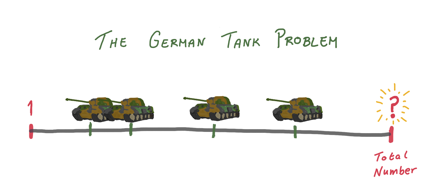
The German Tank Problem

The German tank problem recounts a fascinating story of how the Allies estimated German tank production numbers during World War II.

Early in the war, the Allies started to record the serial numbers on tanks captured from the Germans. The statisticians looking at this data believed that the Germans, being Germans, had numbered their parts in the order they rolled off the production line. Amazingly, using the serial numbers from a relatively small numbers of captured tanks, the statisticians were able to accurately estimate the total number of tanks that were produced! So, how did they do it?

1. Simulations
2. Our first estimator
3. A better estimator
4. Where do these estimators come from?
5. Probabilistic programming

Simulations

Let’s suppose there are 1,000 tanks in total, numbered sequentially from 1 to 1000, and we captured 15 of these tanks uniformly at random. Simulations are a nice way to build intuition around problems in statistics. So, let’s spin up 100,000 parallel universes in our computer to simulate this scenario.

import numpy as np

num_tanks = 1000
num_captured = 15
serial_numbers = np.arange(1, num_tanks + 1)
num_simulations = 100_000

def capture_tanks(serial_numbers, n):
     """Capture `n` tanks, uniformly, at random."""
     return np.random.choice(serial_numbers, n, replace=False)

simulations = [
    capture_tanks(serial_numbers, num_captured)
    for _ in range(num_simulations)
]

The result of each simulation are the serial numbers of the captured tanks, which look something like:

[689, 341, 386, 741, 982, 414, 845, 241, 180, 447, 880,  21, 583, 993, 812]

Our first estimator

Let’s start with a simple estimate for the total number of tanks — the maximum serial number among the captured tanks.

first_estimates = [max(s) for s in simulations]

plt.hist(first_estimates)
avg_first_estimates = np.mean(first_estimates)

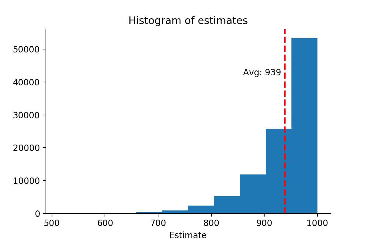
The problem with this estimator is that it will almost always under-estimate the total number of tanks. Indeed, the average estimate across all simulations is 939. In other words, we call this a biased estimator — the expected value of the estimate does not match the true value of the total number of tanks.

A better estimator

Our first estimator is biased, it will tend to under-estimate the true number of tanks. But, what if we could adjust it slightly, taking more information into account? One trait to look at is the spacing between the serial numbers of the captured tanks.

Intuitively, since the tanks are captured uniformly at random, if this spacing is small, then the maximum serial number of captured tanks should be close to the total number of tanks. Conversely, if the spacing between the serial numbers is large, then we should make a larger adjustment to the estimator. With this in mind, an adjusted estimator that I propose is:

(max. serial number) + (average spacing between serial numbers)

The average spacing between serial numbers is1:

(max. serial number) / (num. tanks captured) - 1

Next, let’s try out this new estimator.

def max_plus_avg_spacing(simulation):
    m = max(simulation)
    avg_spacing = (m / num_captured) - 1 
    return m + avg_spacing

new_estimates = [max_plus_avg_spacing(s) for s in simulations]

plt.hist(new_estimates)
avg_new_estimates = np.mean(new_estimates)

Something interesting happens when we make this adjustment to the estimator — the average estimate across all simulations exactly matches the total number of tanks, 1000. In other words, this is an unbiased estimator.

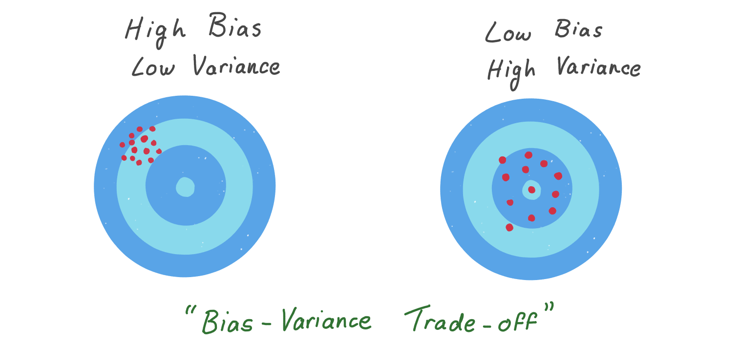
It’s not all rosy however, there is a trade-off in using this estimator. If we look at the standard deviation of the estimates across all simulations for each version:

print(np.std(first_estimates))  #=> 57
print(np.std(new_estimates))    #=> 62

For the first estimator the standard deviation is 57, but for our new adjusted estimator it’s 62. So, while the first estimator will underestimate on average, the distribution is tighter. And while the new estimator is unbiased, there is more variability in its distribution. This is an example of the bias-variance trade-off in action.

Where do these estimators come from?

Altough we built up some intuition to inspire our estimators, they may seem arbitrary. In a way, they are arbitrary — there is no “correct” way to estimate a statistical quantity, just strategies with different benefits and trade-offs. Our first estimator, the maximum serial number of the captured tanks, turns out to be the maximum likelihood estimate (MLE), and its adjustment is the so-called minimum variance unbiased estimator (MVUE). If you’re familiar with the math it’s not too difficult to derive these; but if not, don’t worry, we’ve already covered the intuition surrounding the math.

Probabilistic programming

Until now we have set a fixed value (1000) for the total number of tanks, and used the capture_tanks model to generate simulations. We used these simulations to build intuition around the two estimators we invented, and compared them with metrics like bias and variance. I call this the “simulation” regime, depicted in this diagram:

Back to the real world, suppose 15 tanks were captured with their serial numbers below. Using max_plus_avg_spacing, our estimate for the total number of tanks is 972.

captured = [499, 505, 190, 427, 185, 572, 818, 721, 
            912, 302, 765, 231, 547, 410, 884]

print(max_plus_avg_spacing(captured))   #=> 971.8

But, these estimators we have invented are somewhat ad-hoc. What if we could explicitly reverse the simulation regime? That is, starting from the observed data (the captured serial numbers), simulate the parameters which generated the data according to a probabilistic model. This is called probabilistic programming.

The mechanics of probabilistic programming, while interesting, is too deep to delve into here. Instead, we will jump right into the code using the python library pymc3.

Instead of setting a fixed value for the total number of tanks, with probabilistic programming, we define a prior distribution that encodes our apriori beliefs and knowledge about the parameter(s) of interest. In this case, a reasonable prior distribution for the number of tanks is a DiscreteUniform2 with a lower bound at the maximum serial number of the captured tanks (since it’s impossible for the number of tanks to be lower than this), and an upper bound at some sufficiently large number, say 2000.

With the prior, all that’s left to define is the data-generating distribution, or the likelihood. This is basically just the capture_tanks function from earlier, that we re-define as another DiscreteUniform distribution with pymc3

import pymc3 as pm

with pm.Model():
    num_tanks = pm.DiscreteUniform(
        "num_tanks", 
	lower=max(captured), 
	upper=2000
    )
    likelihood = pm.DiscreteUniform(
        "observed", 
	lower=1, 
	upper=num_tanks, 
	observed=captured
    )
    posterior = pm.sample(10000, tune=1000)

The result of running this model through pymc3 is a large number of samples from the posterior distribution — the probability distribution for the number of tanks given the observed data. The key word here is distribution, rather than a point estimator like the ones we had earlier, we have a distribution that tells us the most credible values for the number of tanks.

pm.plot_posterior(posterior, credible_interval=0.95)

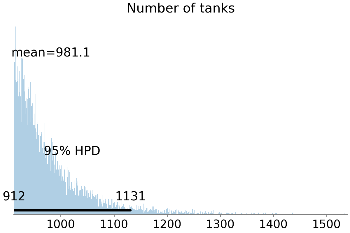
By visualising the posterior distribution, we see its mean value is 981. This value alone is a pretty good estimate for the number of tanks. But we can also use the distribution to tell us more. For example, the 95% highest posterior density (HPD) interval tells us there is a 95% probability that the number of tanks lies somewhere between 912 and 1,131.

Probabilistic programming is a very powerful tool. It’s still a relatively young field, but is starting to become more popular especially due to recent algorithmic advances and an abundance of computational resources. If you’re interested in learning more, Bayesian Methods for Hackers is great resource for beginners. Its main release uses pymc3, but a new version using TensorFlow Probabaility is also available online. For those coming from a stats background, Bayesian estimation supersedes the t-test, blew my mind way back when and opened my eyes to the possibilities of probabilistic programming.

1. This is easiest to see with an example. Suppose the tank serial numbers are [2, 5, 7]. The 4 numbers in the spaces are [1, 3, 4, 6] (remember that the first tank has serial number 1), and so the average spacing in 4/3. ↩

2. For example, a DiscreteUniform(lower=1, upper=10) distribution assigns equal probability to all integers from 1 to 10, and probability 0 to all other numbers. ↩